Modelling can maximize benefits for producers
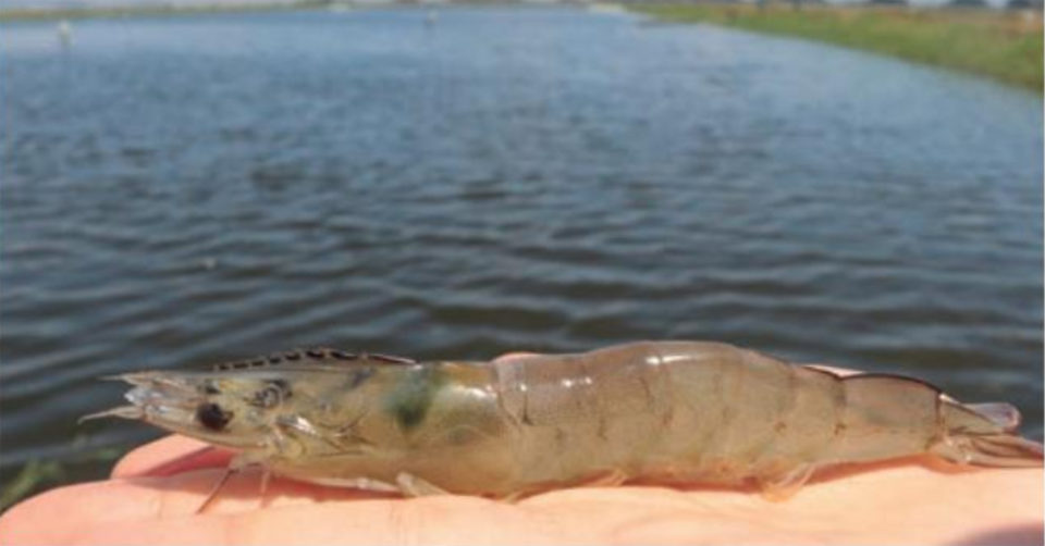
Shrimp aquaculture has a great impact on Ecuador’s national economy. As of July 2018, cumulative shrimp harvests had reached 289,431 metric tons (MT) and $1,868 million in exports.
With the introduction of new technologies, the use of highly specific feeds and genetic improvements, it would be expected that the production cycle would be increasingly shorter and that shrimp growth rates would increasingly come closer to the maximum potential of the animal. This being the scenario, additional efforts are under way to understand the principles that govern the biology of shrimp growth, which is why many of the studies have focused on modeling the increase in size of the Pacific white shrimp (Litopenaeus vannamei) over time.
And an understanding of their growth curves would lead to better administration, management and prediction of a species with such a great aquaculture relevance.
This article (adapted and summarized from the original publication in Revista Acuacultura – Cámara Nacional de Acuacultura, No. 125, October 2018) reviews existing models, which, when adjusted to the physiology of the animal, could have the potential to describe and predict with greater accuracy the feeding behavior of white shrimp.
Models applied to animal production: Empirical relationships
A model is an abstract way of representing reality. The model includes the elements that represent that reality and the relationships between them. In a mathematical model, both variables and functions intervene, logically linked in such a way that the mathematical relationships that govern them correspond to the real-world relationships that they model.
There are several models published for different types of animals, both terrestrial and aquatic. These models relate, for example, the weight and age of different species and breeds. Some of the models used include those of Brody, Von Bertalanffy, Richards, Logistic, and Gompertz. Guinea (1989) reported growth models that include specific equations for rainbow trout, Atlantic salmon, eels, turbot, sole sea bass, sea bream and Japanese seriola. In decapods, growth has also been modeled; which has in common the asymptotic pattern, which means that its growth rate is decreasing as the animal reaches its maximum size.
It is important to distinguish two sub-divisions in the asymptotic growth pattern: sigmoid and exponential. In turn, the sigmoid growth pattern could be Logistic or according to the Gompertz equation, while the exponential is represented by the Von Bertalanffy model. The difference between the Gompertz model and the Logistic one is that in the former one the curve is asymmetric, unlike the latter one where the curve is symmetric. The Gompertz model would best describe the growth of L. vannamei, according to Aragón-Noriega (2016).
Dynamic models: Examples and their application in decapods
Dynamic models are complex models in which the time variable plays a relevant role. In these, the elements that intervene do not remain unchanged, but are functions of time that describe time trajectories that change constantly. Therefore, the objective of a dynamic model is the study of a specific time trajectory of some of its elements.
Dynamic modeling has had several applications in common situations such as transportation. An example of dynamic modeling are air traffic simulation systems, in which the behavior of different types of aircraft can be modeled in scenarios in which not only communication flows in one way but in several. These systems allow the evaluation of algorithms for the management, detection and resolution of conflicts that could occur in very specific situations on a flight.
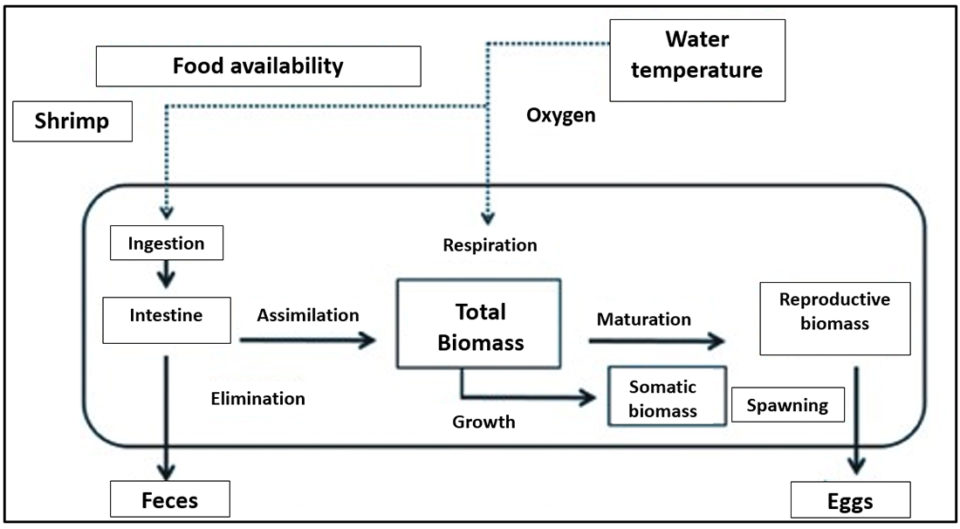
Dynamic models for decapods, on the other hand, mathematically integrate physiological realities in time such as ingestion, assimilation, elimination, respiration and reproduction. These realities, in turn, are governed by the availability of food and temperature. In this type of models, therefore, the demand for food is variable and is adjusted according to the growth of the animal and the parameters of the aquatic environment such as oxygen and temperature (Fig. 1).
All models – being mathematical representations that simplify a phenomenon – require that parameters be estimated. In linear models, the parameters are estimated through the calculation of the ordinate at the origin and the slope. When the models are more complex, the estimation of parameters is done through nonlinear adjustments, which are based on direct-search algorithms.
An algorithm is a sequence of well-defined steps to carry out a process and that clearly indicates what to do in a certain situation. The models applied to animal feeding can be based on algorithms. The algorithms in turn need reference points; for example, consumption sounds, water temperature, dissolved oxygen and others. In the first case, for example, the algorithm will respond in one way or another to the discrimination of the sound of the species in question. For example, the more sound, the more power. In the case of water temperature, the algorithm will respond by varying the power depending on the increase or reduction of the same.
Recently, particle swarm optimization algorithms have been used in aquaculture. This type of algorithm works with a set of candidate solutions that move in the search space, following logical-mathematical rules that define better or worse positions. As potential solutions are found, the “swarm” moves toward them in a process that repeats a finite number of times. If in this swarm movement process there are particles that detect solutions that could represent an optimum, the swarm will reorient the position. Just as a group of bees seek regions with a higher concentration of flowers, this algorithm considers both the experience of each particle and the whole.
The technological tools applied to animal production and feeding can be based on algorithms that have been increasing their degree of complexity over time. For this reason, several algorithms have been applied to different areas, such as food formulation, food production, fish production, and pumping optimization. Algorithms are the fundamental pillars that support the concept of precision feeding.
Dynamic models for shrimp can define the growth, feeding and survival of the animal based on changing environmental conditions. Among the implications is, for example, the daily adjustment of the ration, unlike the common practice through which the ration is changed once a week. These models are of specific application and, therefore, have to be implemented at productive unit, that is, at each shrimp grow-out pond.
Field assessments
In order to demonstrate the use of models in real situations, the calculation and dispersion of feed in automated feeding was put to the test under different climatic and environmental conditions. One of these tests was conducted at a shrimp farm located in El Morro, with earthen ponds stocked at densities of between 90,000 and 200,000 shrimp per hectare. The installed pumping capacity of the shrimp farm allowed a daily water exchange of approximately 10 percent.
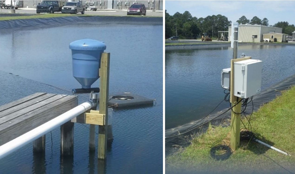
The feed was dispersed throughout the day with three automatic feeders in timer mode, located under certain technical criteria and 50 m apart in a 3-hectare (ha) pond. The amount of feed was calculated daily by means of a precision aquaculture system and according to the environmental conditions of the day (oxygen, temperature, pH).
On a weekly basis, the program received information regarding shrimp weights and salinity. Table 1 shows the results of the first cycle, obtained without feeding automation, and feeding a nutritionally complete feed based on a feeding table. In this scheme, feeding was performed twice a day, while during three subsequent cycles ponds were fed 24 hours with the same feed using automatic feeders and calculating the feed adjustments using the precision aquaculture system.
Molina, algorithms, Table 1
| Parameters | Cycle 1 | Cycle 2 | Cycle 3 | Cycle 4* |
|---|
Parameters | Cycle 1 | Cycle 2 | Cycle 3 | Cycle 4* |
|---|---|---|---|---|
| Initial density (shrimp/ha) | 90,000 | 105,000 | 200,000 | 140,000 |
| Final density (shrimp/ha) | 15,900 | 73,500 | 95,600 | 93,800 |
| Survival (%) | 51 | 70 | 48 | 67 |
| Production (pounds/ha) | 2,774 | 2,871 | 4,400 | 4,404 |
| Performance (pounds/ha/day) | 23 | 35 | 46 | 57 |
| Final weight (grams) | 22 | 18 | 21 | 22 |
| Cumulative growth (grams/week) | 1.3 | 1.5 | 1.7 | 1.8 |
| FCR | 1.6 | 1.6 | 1.4 | 1.5 |
| Production days | 119 | 82 | 86 | 76 |
| Profit ($/ha/day) | 15 | 31 | 38 | 57 |
| Feeding frequency | 2 X day | Multiple 24 hr | Multiple 24 hr | Multiple 24 hr |
| Feeding method | Manual | Automatic | Automatic | Automatic |
| Mechanical aeration (diesel) | – | – | 16.6 hp/ha | 16.6 hp/ha |
The feeding results for cycle 2, following the precision aquaculture system, showed an increase of around 42 and 16 percent in survival rates (51 vs. 70 percent) and growth (1.3 vs 1.5 grams/week) respectively, compared to the first cycle of the pond. A reduction of around 37 days of the production cycle with the use of automated feeding was also observed. The feed conversion factor (FCR) was similar between the two cycles, although somewhat high due to observed mortalities of large shrimp during the last weeks of the cycle and due to diseases.
The automatic calculation of feeding and feed dispersion were repeated during two consecutive cycles (3 and 4), but this time incorporating mechanical aeration. Regardless of the stocking densities (200,000 and 140,000 shrimp/ha), the harvest densities were very similar, as well as the harvested biomass of around 4400 pounds per ha. The main difference between these two cycles was the highest profit achieved ($57 vs. $38/ha/day by cycles 4 and 3, respectively). This was due to having stocked larger (2.7 grams) shrimp in cycle 4, which reduced its duration by 10 days. In addition, it is important to consider that there were oxygen drops and outbreaks of vibriosis during the cycle. The FCRs were similar to the previous cycles, which demonstrates the functionality of the precision aquaculture system.
Another study was carried out at two shrimp farms located in Las Esclusas and Churute, where earthen ponds where stocked at a density between 130,000 and 220,000 shrimp per hectare. The first farm had a daily water exchange of approximately 10 to 12 percent, while the other shrimp farm used recirculation.
The feed was dispersed in each pond throughout the day in shrimp farm 1 with one automatic feeder in timer mode for every 2 hectares, while in shrimp farm 2 one feeder was used per each hectare. The precision aquaculture system provided the daily amount of feed that was distributed according to the environmental conditions of the day (oxygen, temperature, salinity, pH).
The collected field data, comparing the historical data vs. the resulting data using the precision aquaculture system, are summarized in Table 2. The results show an increase of between 90 and 144 percent in the biomass (lbs.) harvested in the ponds that were fed according to the precision aquaculture system. The yields (pounds/ha/day) in both shrimp farms were more than double when compared to those resulting from traditional management, regardless of the salinity and whether the production system was open or closed. This was mainly due to greater survival. A better feed conversion was also observed, more evident in the shrimp farm that was operated with an open water exchange system.
Molina, algorithms, Table 2
| Parameters | Reference Case 1 | Shrimp Farm 1 SAP* | Reference Case 2 | Shrimp Farm 2 SAP* |
|---|
Parameters | Reference Case 1 | Shrimp Farm 1 SAP* | Reference Case 2 | Shrimp Farm 2 SAP* |
|---|---|---|---|---|
| Initial density (shrimp/ha) | 11 | 18 | 11 | 23 |
| Final density (shrimp/ha) | 5 | 7 | 4 | 11 |
| Survival (%) | 46 | 41 | 35 | 47 |
| Production (pounds/ha) | 2,011 | 3,824 | 1,485 | 3,628 |
| Performance (pounds/ha/day) | 16 | 32 | 15 | 33 |
| Final weight (grams) | 17.1 | 19.8 | 17.0 | 15.8 |
| Cumulative growth (grams/week) | 0.96 | 1.17 | 1.27 | 1.00 |
| FCR | 3.1 | 2.4 | 2.47 | 2.35 |
| Production days | 126 | 118 | 98 | 109 |
| Salinity (ppt) | 29-30 | 29-30 | 2-9 | 2-9 |
| Production system | Open | Open | Closed | Closed |
| Sector | Las Esclusas | Las Esclusas | Churute | Churute |
| Number of ponds | 12 | 11 | 16 | 10 |
Perspectives
The data generated in three different sectors and management conditions reinforces the fact that the precision aquaculture system is a modeling tool to calculate the daily amount of feed that – together with a nutritionally complete feed and an adequate feeding strategy – helps exceed the profits that can be obtained with a traditional diet based on calculating the amount of weekly feed using a table based on percentages of the estimated biomass.
The precision aquaculture system has a lot of potential to define new feeding strategies, which would mean a sustainable saving that would allow maximizing productive results at a minimum cost. The application of new tools requires a technological change at the farm. The continuous monitoring of parameters is one of the requirements to obtain a greater benefit from these new tools.
Automatic feeding, capable of dividing the feed ration into variable quantities throughout the day, is also a requirement without which the use of models loses meaning. This change does not necessarily require an excessive investment.
With the use of these models, it will be increasingly common to be able to describe and predict growth, food consumption, survival, harvest and various other parameters under specific conditions. In this way, cost-benefit evaluations can be provided in various production scenarios. According to these valuations and the production objectives of the farms, the models would provide a series of recommendations, including the selection of the most profitable feed and the best strategy, which will allow producers to achieve maximum benefits, even more so in the current shrimp price crisis.
References available from the first author.
Authors
-
-
Manuel Espinoza, M.Sc.
Investigación y Desarrollo
Skretting Ecuador
Tagged With
Related Posts
Innovation & Investment
Acoustic control improves feeding productivity at shrimp farms
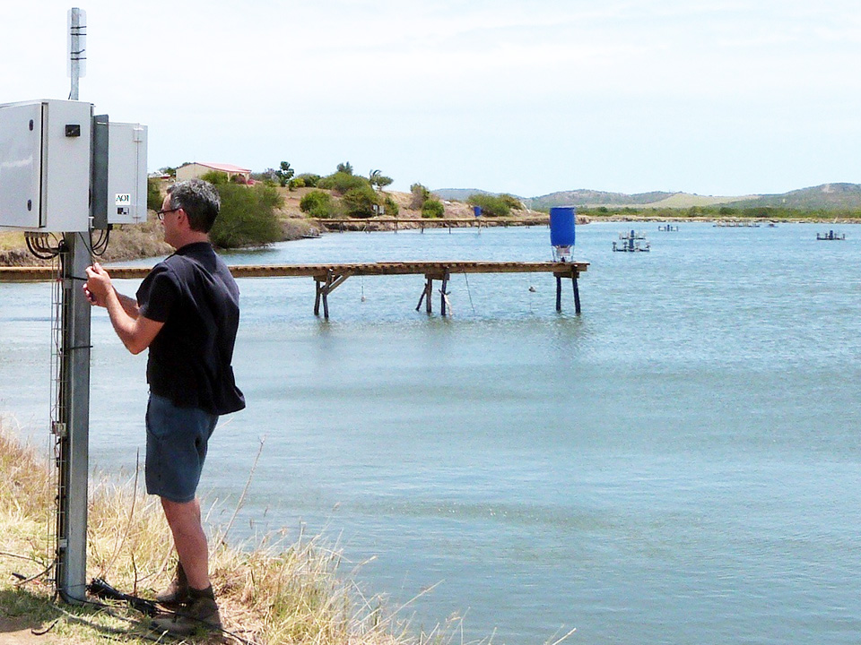
In systems recently developed for shrimp farms, passive acoustic-based technology enables sensor-based control of multiple automatic feeders. Improved growth and feed conversion have been recorded at commercial farms using the technology.
Innovation & Investment
Can IoT tool help fish farmers sleep better at night?
Berlin-based Monitorfish wants to enable fish farmers to keep a close watch on their stocks from their smartphones, another Internet of Things solution for producers.
Aquafeeds
Automated feeding systems in pond production of Pacific white shrimp
Results of this study show that automated feeding systems are significantly more efficient than hand feeding in shrimp production ponds and that increases in feed input, application of adaptive technology and training of people to maintain the feeding system must all be considered.
Innovation & Investment
Fish behavior-tracking tech aims to curb aquafeed wastage
Overfeeding is a waste stream for aquaculture. Underwater cameras in pens help, but a company mixing hydroacoustics and machine learning has another idea.


